Derivation of the Poisson Distribution
This post contains my notes from trying to understand where the Poisson distribution comes from.
Interlude on limit definition of $\exp$
To start out, let’s understand the definition that is commonly given for $e$:
\[e:= \lim_{x\to\infty} \left(1 + {1 \over x}\right)^x\]It’s probably better to think of this in terms of $e^x$, exponentiation. Consider:
\[\exp(y) := \lim_{x\to\infty} \left(1 + {y \over x}\right)^x\]The existence of this limit can be shown by Bernoulli’s inequality. Now note:
- $\exp(0)=1$
- $\exp(a\cdot b)=(\exp(a))^b$
- $\exp(a + b) = \exp(a) \cdot \exp(b)$
- ${d \over dx} \exp(x) = \exp(x)$
(1) follows immediately from the definition.
To show (2), we have:
\[\begin{aligned} \exp(ab) & = \lim_{x\to\infty} \left(1 + {ab \over x}\right)^x \\ & = \lim_{q\to\infty} \left(1 + {a \over q}\right)^{b\cdot q} \quad \left(\textrm{substitute } q=x/b\right) \\ & = \left(\lim_{q\to\infty} \left(1 + {a \over q}\right)^q\right)^b \\ & = \left(\exp(a)\right)^b \\ \end{aligned}\]For (3):
\[\begin{aligned} \exp(a+b) & = \lim_{x\to\infty} \left(1 + {a+b \over x}\right)^x \\ & = \lim_{q\to\infty} \left(1 + {1 \over q}\right)^{q\cdot (a+b)} \quad \left(\textrm{substitute } q={x\over a+b}\right) \\ & = \left(\lim_{q\to\infty} \left(1 + {1 \over q}\right)^q\right)^{a+b} \\ & = \left(\exp(1)\right)^{a+b} \\ & = \exp(1)^a\cdot \exp(1)^b \\ & = \exp(a)\cdot \exp(b) \\ \end{aligned}\]For (4), we have:
\[\begin{aligned} {d \over dx} \exp(x) &= \lim_{\delta\to 0} \frac{\exp(x+\delta) - \exp(x)}{\delta} \\ &= \lim_{\delta\to 0} \frac{\exp(x)\exp(\delta) - \exp(x)}{\delta} \\ &= \exp(x)\left(\lim_{\delta\to 0} \frac{\exp(\delta) - 1}{\delta} \right) \\ &= \exp(x)\left(\lim_{\delta\to 0} \frac{\left(\lim_{y\to\infty}(1 + 1/y)^y\right)^\delta - 1}{\delta} \right) \\ &= \exp(x)\left(\lim_{\delta\to 0} \frac{\left((1 + \delta)^{1\over \delta}\right)^\delta - 1}{\delta} \right) \quad \left(\textrm{letting }y=1/\delta\right)\\ &= \exp(x)\left(\lim_{\delta\to 0} \frac{(1 + \delta) - 1}{\delta} \right) \\ &= \exp(x)\left(\lim_{\delta\to 0} \frac{\delta}{\delta} \right)\\ &= \exp(x) \\ \end{aligned}\]Poisson (as a limit of Binomial)
Note: follows this post.
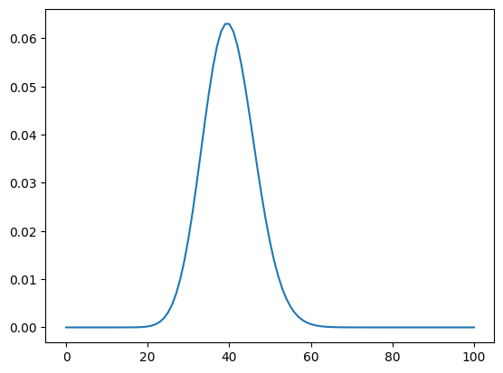
As a motivating example, consider the number of customers to a grocery store in a town, where every person in the town has probability $p$ of going to the store during a particular hour. Suppose there are 40,000 people in the town, and they each have a 1/1,000 chance of going to the store during that hour.
The PMF for this looks like:
import scipy.stats, numpy as np
n = 100
xs = np.linspace(0, n, n + 1)
ys = scipy.stats.binom.pmf(xs, 40_000, 1 / 1_000)

import matplotlib.pyplot as plt

plt.plot(xs, ys)
plt.show()
Now suppose we have $n$ binomial trials in a given time period, but we do not know $n$ or the parameter $p$. We only know the expected number of successes during that time period, $\lambda$. (In the example above, we don’t know how many people shop at this store, nor how likely they are to do so at 6-7pm on a Saturday.) But note that whatever $n$ and $p$ are, we have:
\[\lambda = np\]Or, equivalently:
\[p = {\lambda \over n}\]Then since this is a binomial trial, we have:
\[P(X=k) = {n \choose k} \left({\lambda \over n}\right)^k \left(1 - {\lambda \over n}\right)^{n-k} = {n! \over k!(n-k)!} \left({\lambda \over n}\right)^k \left(1 - {\lambda \over n}\right)^{n-k}\]Taking the limit as $n\to\infty$:
\(\begin{aligned} P_\infty(X=k) &= {\lambda^k \over k!} \cdot \lim_{n\to\infty} {n! \over (n-k)!} \left({1 \over n}\right)^k \left(1 - {\lambda \over n}\right)^{n-k} \\ &= {\lambda^k \over k!} \cdot \lim_{n\to\infty} {n! \over n^k(n-k)!} \left(1 - {\lambda \over n}\right)^n\left(1 - {\lambda \over n}\right)^{-k} \\ & \textrm{Canceling like terms, we end up with }k\textrm{ terms of size }O(n)\textrm{ on top and bottom, so the first term is 1. Thus:} \\ &= {\lambda^k \over k!} \cdot \lim_{n\to\infty} \left(1 - {\lambda \over n}\right)^n\left(1 - {\lambda \over n}\right)^{-k} \\ & \textrm{Since }k\textrm{ is fixed. The second term is 1:} \\ &= {\lambda^k \over k!} \cdot \lim_{n\to\infty} \left(1 - {\lambda \over n}\right)^n \\ &= {\lambda^k e^{-\lambda} \over k!} \\ \end{aligned}\) That is the standard PMF of the Poisson distribution. In our example above, we have $\lambda=40$:
import scipy.stats, numpy as np, scipy.special
bound = 100
λ = 40
xs = np.linspace(0, bound, bound + 1)
ys = np.power(λ, xs) * np.exp(-λ) / scipy.special.factorial(xs)

import matplotlib.pyplot as plt

plt.plot(xs, ys)
plt.show()
